Visual Demos for Theoretical Results (in Human Computation)

A sub-area of computer science, where a large part of my own work lies, is on theoretical topics in human computation. A broad class of questions here involve a set of items, and data in the form of evaluations of these items made by humans. The goal is to infer certain properties about these items based on this data from people. The research involves designing algorithms, proving mathematical guarantees, and also running experiments. The results are usually in the form of theorems, proofs, tables or plots. However, these forms of results are not nearly as impactful as a visual demonstration like in computer vision, particularly to an audience that may be short on time or may not have sufficient expertise. So can we make some of these results visually exciting, showing the algorithms “in action,” by using cute cat pictures?

Yes indeed! The idea is to use this mapping:

Actual	Visual
Set of items	An image
Each item	Pixel in the image
True value of item (unknown to algorithm)	Value of pixel
Noisy/biased item evaluation by people	Noisy/biased function of pixel generated via human computation models
Algorithm to estimate values of these items based on these estimates	The same algorithm now estimates the values of the pixels
Theorem/proof/table/plot	Reconstructed image using estimated pixel values!

Here are some illustrations using three popular problem settings in this field: (i) ranking and preference learning, (ii) miscalibration, (iii) commensuration bias or subjectivity, and (iv) crowdsourced labeling.

(I) Ranking and Preference Learning

You have a collection of items, and each item has some unknown true “value”. People are asked to compare pairs of these items and tell us which one they think has the higher value. Based on this data from people, the goal is to estimate these values. There are various models proposed in the literature for the noise in human evaluations (e.g., the Thurstone and BTL models) and algorithms for estimation (e.g., maximum likelihood estimates or MLEs under these models). See [1], [2] for more details on this problem setting.

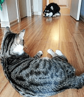
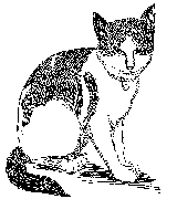
We’ll visually evaluate them using this image (true values):

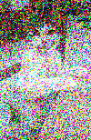
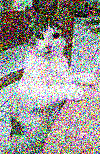
The following visuals illustrate the consistency property: if the comparisons are generated via the Thurstone model, then given a large enough number of pairwise comparisons, the output of the Thurstone MLE will come arbitrarily close to the true values. Here are the reconstructed images as we increase the number of pairwise comparisons available:

We now visualize issues of model mismatch, where the data is generated from one model but the estimation algorithm assumes a different model. The table below shows generation and estimation from the Thurstone and the Bradley-Terry-Luce model. One can see that the quality of estimation is similar in all four cases — the visuals indeed reflect the reality that the actual error in all four cases are comparable.

Estimation algorithm → Generation model ↓	Thurstone MLE	BTL MLE
Thurstone
Bradley-Terry-Luce

Here is the associated code which you can feel free to play around with.

(II) Miscalibration

Consider the application of scientific peer review. A collection of papers are submitted to a conference, and each paper is evaluated by a small number of reviewers. The evaluations typically comprise a score. A key problem with scores is that of miscalibration of reviewers: some reviewers are lenient, some strict, some are extreme, some moderate, and so on. The goal is to recalibrate their scores, without any prior knowledge of the miscalibration of any reviewer.

Here we consider each pixel as a paper and evaluate the effects of miscalibration. Original image (true values):

https://upload.wikimedia.org/wikipedia/commons/thumb/8/8e/Domestic_cat_watching_an_alaskan_malamute.jpg/340px-Domestic_cat_watching_an_alaskan_malamute.jpg

We first assume an “affine” miscalibration, meaning that each reviewer is associated to three randomly drawn parameters (a, b, c) in [0,1] which sum to 1. The score given by a reviewer is a convex combination via that reviewer’s parameters: a*true score + b*1 + c*0. If every paper (pixel) is reviewed by one reviewer, and if every reviewer reviews 5 papers, then here is what the (miscalibrated) scores look like:

We now recalibrate the scores by simply normalizing the mean and standard deviation of each reviewer, setting them equal to the true mean and standard deviation of the entire image. Then we get the recalibrated image:

That’s actually pretty good! Now, a lot of literature assumes such affine miscalibration, and proposes algorithms for recalibration. But the miscalibration in humans is more complex, and this is where things get messy.

Now consider this miscalibration: if the value is greater than some threshold, then scale it down (by a reviewer-dependent factor) to near that threshold, otherwise leave it as is. This miscalibration represents reviewers who are fine with lower-score papers but are stingy in giving good scores to better papers. Here is the miscalibrated image:

Here is the recalibrated image we get after normalizing the mean and standard deviation for each reviewer:

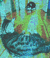
As you can see, the recalibration in this case is not really as good as that in the affine miscalibration setting. In fact, dealing with more complex miscalibration is an important open problem. See [3] for more details. And here is the associated code which you can feel free to play around with.

(III) Commensuration Bias or Subjectivity

Let us continue with our peer review application. Another key challenge is that of commensuration bias (or subjectivity): different reviewers have personal, subjective preferences on how to weigh different criteria to make the final decision. For instance, one reviewer may put a high emphasis on novelty whereas another may emphasize empirical performance — then a novel paper with mediocre empirical performance would be accepted if reviewed by the first reviewer and rejected if by the second reviewer based solely on the personal preference of the reviewer on how to weigh novelty versus empirical results. The goal is to mitigate this arbitrariness in the peer review process.

Suppose each pixel in this image is a review. Each review comprises evaluations along three criteria, represented by the values of the red, green, and blue components (think of red representing novelty, green the empirical performance, and blue representing clarity of writing).

https://upload.wikimedia.org/wikipedia/en/thumb/f/ff/Cattanooga_Cats.jpg/250px-Cattanooga_Cats.jpg

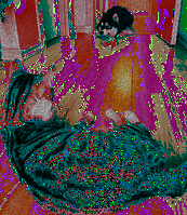
For any review, the reviewer combines the individual criteria evaluations to form an overall recommendation. Each reviewer has their own personal subjective preference on how to do this. In this visualization we assume that each overall recommendation is a convex combination of individual criteria evaluations, where the coefficients are specific to the reviewer. The overall recommendations are::

As you can see, this subjectivity has made the overall recommendations quite messy and inconsistent.

We use the algorithm in [4] to “learn” a function that maps criteria evaluations to overall recommendations, where this function is an aggregate of the individual mappings used by all reviewers. Applying this mapping to the criteria scores in all reviews, we get a re-adjusted overall recommendations, which appears more appealing:

See [4] for more background and details on commensuration bias. Feel free to play around with the code here.

(IV) Crowdsourced Labeling

Each item is a (binary choice) question. Each question is asked to multiple workers, who give possibly erroneous responses. The goal is to estimate the correct answer to each question.

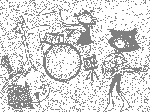
Consider this image with each pixel (black or white) representing a binary-choice question:

https://upload.wikimedia.org/wikipedia/commons/thumb/2/2d/Nansen_%28cat%29.jpg/120px-Nansen_%28cat%29.jpg

Let’s suppose there are 10 workers and each worker answers all questions. Five of these workers are correct on any question with a 90% chance, and the five remaining workers are correct on any question with a 60% chance.

A popular algorithm for estimating the correct answers is to take a majority vote over all workers for each question. Unlike many other algorithms in the literature, this simple algorithm is extremely robust to modeling assumptions. Here is its performance:

Majority voting will, however, perform poorly if there are many workers who are largely guessing the answers. An alternative approach in [5] is to identify an appropriate set of “knowledgable” workers in a data-dependent manner and take a majority vote of only these workers. Here we consider an “idealized” version of such an algorithm which correctly knows identities of knowledgable workers. Taking a majority vote of only these workers, we get:

See [5] for more details on crowdsourced labeling. And here is the associated code which you can feel free to play around with.

All in all, if you work in related areas, we hope some of these ideas will be useful to make an impact via visual demonstrations in your next presentation, blog, etc.

References

[1] “Estimation from Pairwise Comparisons: Sharp Minimax Bounds with Topology Dependence,” N. Shah, S. Balakrishnan, J. Bradley, A. Parekh, K. Ramchandran, and M. Wainwright, 2016.
[2] “Stochastically Transitive Models for Pairwise Comparisons: Statistical and Computational Issues.” N. Shah, S. Balakrishnan, A. Guntuboyina, and M. Wainwright, 2017.
[3] “Your 2 is My 1, Your 3 is My 9: Handling Arbitrary Miscalibrations in Ratings,” J. Wang and N. Shah, 2019.
[4] “Loss functions, axioms, and peer review,” R. Noothigattu, N. Shah, and A. Procaccia, 2020.
[5] “A Permutation-based Model for Crowd Labeling: Optimal Estimation and Robustness,” N. Shah, S. Balakrishnan, and M. Wainwright, 2016.
This is fantastic!